9 Data Sets
Chapter 9 demonstrates several, though not all, data objects from package datasets (R version 4.5.3 (2026-03-11)) and package spatstat.data (v3.1.9, GPL (>= 2)).
The function calls in Chapter 9 are exclusively those provided in package base and stats (R version 4.5.3 (2026-03-11)), and in the spatstat.* family of packages.
9.1 anemones
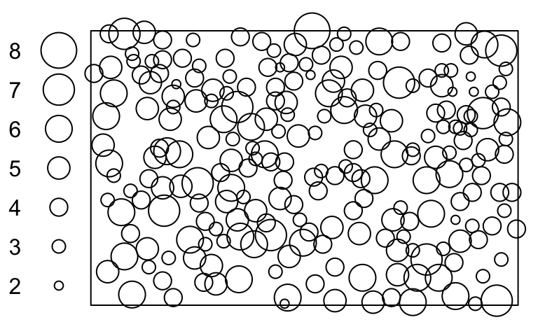
The point-pattern (ppp.object, Chapter 24) anemones from package spatstat.data (v3.1.9, GPL (>= 2)) has (Listing 9.2, Figure 9.1)
- 231 points (Listing 9.3);
- rectangle observation window (Chapter 22, Listing 9.4);
- one integer-mark (Listing 9.5);
'vector'mark-format (Listing 9.6).
anemones
Code
par(mar = c(0,0,0,0))
spatstat.data::anemones |>
spatstat.geom::plot.ppp(main = NULL)anemones
anemones
spatstat.data::anemones |>
  spatstat.geom::print.ppp()
Marked planar point pattern: 231 points
marks are numeric, of storage type 'integer'
window: rectangle = [0, 280] x [0, 180] unitsanemones
spatstat.data::anemones |>
  spatstat.geom::npoints.ppp()
[1] 231anemones
spatstat.data::anemones |>
  spatstat.geom::Window.ppp()
window: rectangle = [0, 280] x [0, 180] unitsanemones
spatstat.data::anemones |>
  spatstat.geom::marks.ppp() |>
  typeof()
[1] "integer"anemones
spatstat.data::anemones |>
  spatstat.geom::markformat.ppp()
[1] "vector"9.2 ants
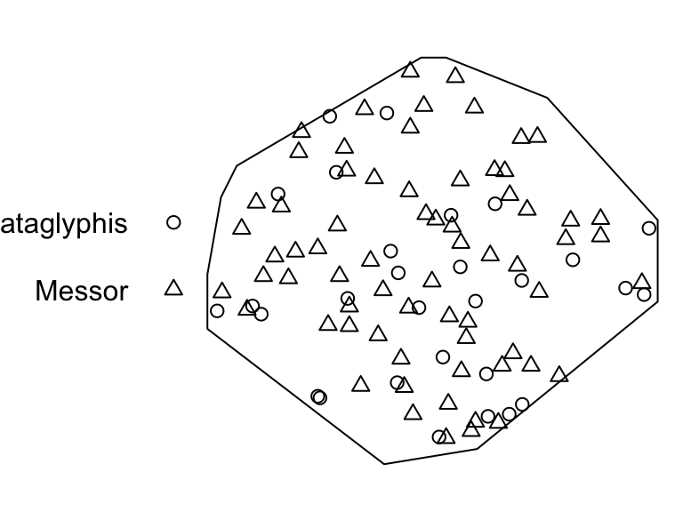
The point-pattern (ppp.object, Chapter 24) ants from package spatstat.data (v3.1.9, GPL (>= 2)) has (Listing 9.8, Figure 9.2)
- 97 points;
- polygonal window;
- one multi-type mark with two levels,
'Cataglyphis'and'Messor'(Listing 9.9); 'vector'mark-format.
ants
Code
par(mar = c(0,0,0,0))
spatstat.data::ants |>
spatstat.geom::plot.ppp(main = NULL)ants
ants
spatstat.data::ants |>
  spatstat.geom::print.ppp()
Marked planar point pattern: 97 points
Multitype, with levels = Cataglyphis, Messor
window: polygonal boundary
enclosing rectangle: [-25, 803] x [-49, 717] units (one unit = 0.5 feet)ants
spatstat.data::ants |>
  spatstat.geom::marks.ppp() |>
  table()
Cataglyphis      Messor
         29          68
9.3 austates
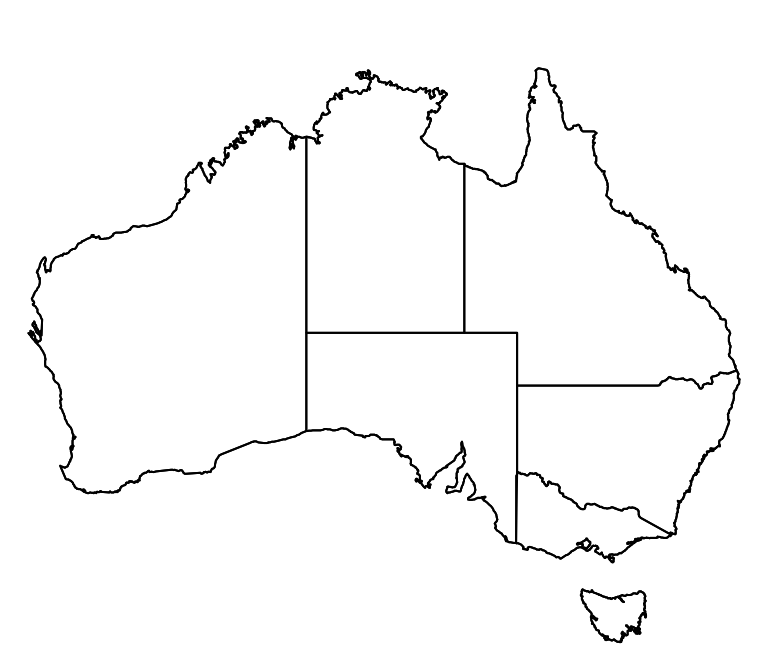
The tessellation (Chapter 29) austates from package spatstat.data (v3.1.9, GPL (>= 2)) has (Listing 9.11, Figure 9.3)
- 7 tiles (Listing 9.12);
- polygonal window;
- no marks.
austates
Code
par(mar = c(0,0,1,0))
spatstat.data::austates |>
spatstat.geom::plot.tess(main = '')austates
austates
spatstat.data::austates |>
  spatstat.geom::print.tess()
Tessellation
Tiles are irregular polygons
7 tiles (irregular windows)
window: polygonal boundary
enclosing rectangle: [113.19392, 153.6692] x [-43.59316, -10.93156] degreesaustates
spatstat.data::austates |>
  spatstat.geom::tiles()
List of spatial objects
WA:
window: polygonal boundary
enclosing rectangle: [113.19392, 129.01141] x [-35.11407, -13.76426] degrees
NT:
window: polygonal boundary
enclosing rectangle: [129.01141, 138.0038] x [-25.988593, -11.045627] degrees
SA:
window: polygonal boundary
enclosing rectangle: [129.01141, 141.0076] x [-37.96578, -25.98859] degrees
QLD:
window: polygonal boundary
enclosing rectangle: [138.0038, 153.47909] x [-29.163498, -10.931559] degrees
NSW:
window: polygonal boundary
enclosing rectangle: [141.0076, 153.6692] x [-37.45247, -28.07985] degrees
VIC:
window: polygonal boundary
enclosing rectangle: [140.95057, 149.79087] x [-39.04943, -33.91635] degrees
TAS:
window: polygonal boundary
enclosing rectangle: [144.63878, 148.34601] x [-43.59316, -40.58935] degrees9.4 betacells
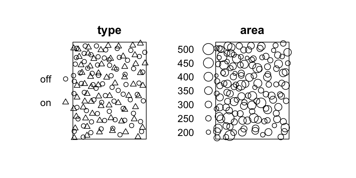
The point-pattern (ppp.object, Chapter 24) betacells from package spatstat.data (v3.1.9, GPL (>= 2)) has (Listing 9.14, Figure 9.4)
- 135 points;
- rectangle window;
'dataframe'mark-format (Listing 9.15);- one numeric mark
area(Listing 9.16); - one multi-type mark
typewith two levels,'off'and'on'(Listing 9.16).
betacells
Code
par(mar = c(0,0,0,0))
spatstat.data::betacells |>
spatstat.geom::plot.ppp(main = '')betacells
betacells
spatstat.data::betacells |>
  spatstat.geom::print.ppp()
Marked planar point pattern: 135 points
Mark variables: type, area
window: rectangle = [28.08, 778.08] x [16.2, 1007.02] micronsbetacells
spatstat.data::betacells |>
  spatstat.geom::markformat.ppp()
[1] "dataframe"betacells
spatstat.data::betacells |>
  spatstat.geom::marks.ppp()
type area
1 on 275.9
2 off 241.2
3 on 256.0
4 on 442.9
5 off 209.4
6 off 260.4
7 on 348.8
8 on 315.2
9 off 275.3
10 off 317.8
11 on 310.0
12 off 279.4
13 on 375.3
14 off 307.3
15 on 378.2
16 on 286.9
17 off 303.0
18 off 202.4
19 off 277.3
20 off 278.8
21 on 244.1
22 on 341.5
23 off 322.5
24 off 248.4
25 off 319.9
26 on 315.5
27 off 353.1
28 on 514.4
29 on 404.2
30 on 360.4
31 on 252.8
32 off 276.1
33 off 274.4
34 off 251.7
35 off 298.9
36 on 370.0
37 on 207.9
38 off 257.2
39 on 325.4
40 off 310.0
41 on 305.0
42 on 317.0
43 on 373.5
44 on 435.1
45 on 366.8
46 off 245.5
47 on 276.1
48 off 268.9
49 off 252.2
50 off 227.4
51 off 319.0
52 on 320.5
53 on 327.2
54 on 384.6
55 on 285.8
56 on 321.3
57 off 245.5
58 off 245.2
59 off 256.0
60 on 303.8
61 off 225.4
62 off 294.2
63 off 244.4
64 off 257.2
65 off 199.5
66 on 263.3
67 on 345.5
68 on 279.9
69 on 427.8
70 off 239.4
71 off 249.3
72 on 228.3
73 off 320.5
74 on 340.9
75 off 257.8
76 on 363.3
77 off 274.4
78 off 246.7
79 on 348.2
80 on 350.5
81 on 287.2
82 off 258.6
83 off 168.3
84 off 260.7
85 off 263.9
86 on 286.1
87 off 189.0
88 off 220.4
89 on 345.3
90 on 345.5
91 off 308.8
92 off 257.5
93 off 258.4
94 on 412.3
95 off 235.0
96 on 273.8
97 on 312.9
98 off 302.1
99 on 391.3
100 off 266.2
101 on 362.2
102 off 243.2
103 on 360.1
104 on 224.8
105 off 209.4
106 off 239.4
107 off 242.3
108 on 377.3
109 on 255.7
110 off 173.5
111 off 198.3
112 off 223.4
113 on 439.7
114 off 219.3
115 on 281.7
116 off 214.3
117 on 291.9
118 off 231.5
119 on 323.1
120 off 262.4
121 off 342.0
122 off 195.4
123 on 274.4
124 off 278.2
125 on 293.6
126 off 254.6
127 off 286.1
128 on 233.6
129 on 337.4
130 on 345.5
131 off 360.1
132 off 285.2
133 on 305.9
134 on 229.8
135 on 251.79.5 bronzefilter
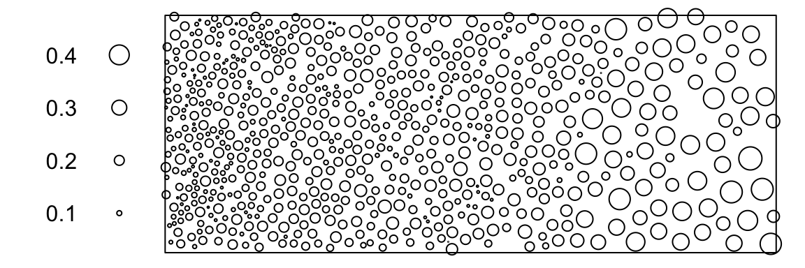
The point-pattern (ppp.object, Chapter 24) bronzefilter from package spatstat.data (v3.1.9, GPL (>= 2)) has (Listing 9.18, Figure 9.5)
- 678 points;
- rectangle window;
- one numeric mark.
bronzefilter
Code
par(mar = c(0,1,0,0))
spatstat.data::bronzefilter |>
spatstat.geom::plot.ppp(main = NULL)bronzefilter
bronzefilter
spatstat.data::bronzefilter |>
  spatstat.geom::print.ppp()
Marked planar point pattern: 678 points
marks are numeric, of storage type 'double'
window: rectangle = [0, 18] x [0, 7] mm9.6 btb.extra
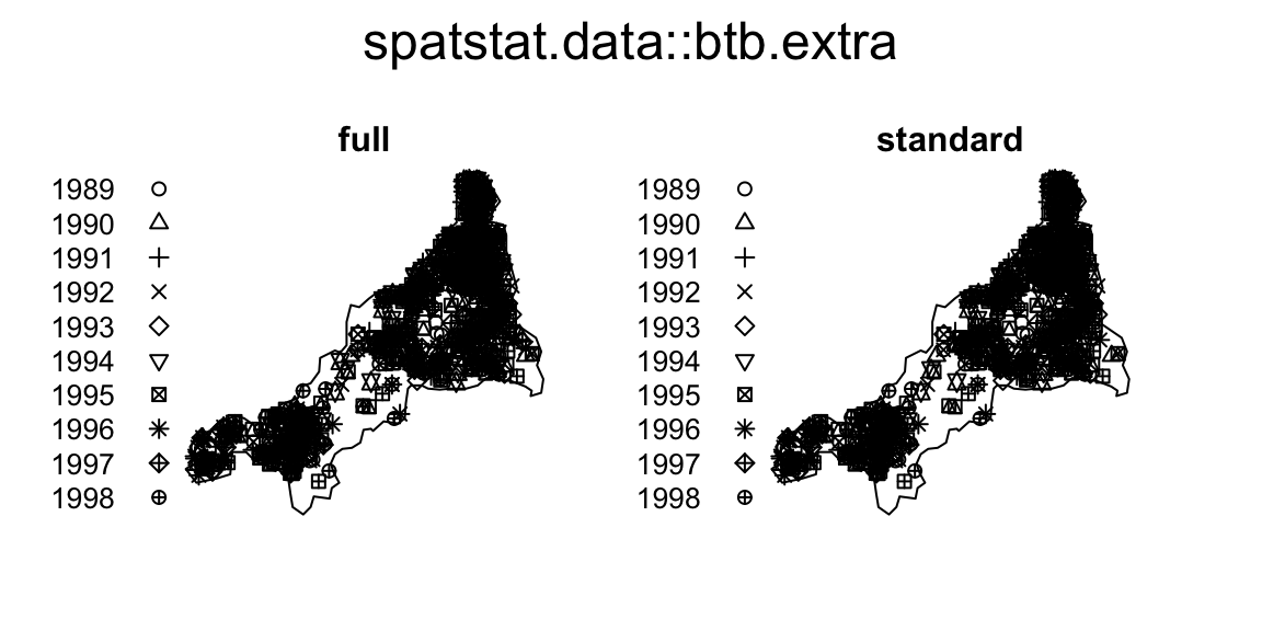
The point-pattern-list (ppplist, Chapter 25) btb.extra from package spatstat.data (v3.1.9, GPL (>= 2)) (Listing 9.20, Figure 9.6)
- inherits from the
S3class'solist'(Chapter 27, Listing 9.21); - contains 2 point-pattern (
ppp.object, Chapter 24) members (Listing 9.22).
btb.extra
Code
par(mar = c(0,1,1,1))
spatstat.data::btb.extra |>
spatstat.geom::plot.solist()btb.extra
btb.extra
spatstat.data::btb.extraList of point patterns
full:
Marked planar point pattern: 919 points
Mark variables: year, spoligotype
window: polygonal boundary
enclosing rectangle: [133.5147, 246.0193] x [10.88514, 118.7298] km
standard:
Marked planar point pattern: 873 points
Mark variables: year, spoligotype
window: polygonal boundary
enclosing rectangle: [133.5147, 246.0193] x [10.88514, 118.7298] kmbtb.extra
spatstat.data::btb.extra |>
  class()
[1] "ppplist" "solist" "anylist" "listof" "list" class of members of btb.extra
spatstat.data::btb.extra |>
  sapply(FUN = class)
full standard
"ppp" "ppp" 9.7 cars
The data frame (data.frame, Chapter 12) cars from package datasets (R version 4.5.3 (2026-03-11)) has (Listing 9.23)
- 50 rows and 2 columns (Listing 9.24)
- two numeric columns:
$speedand$dist.
cars
datasets::cars |>
  print.data.frame()
speed dist
1 4 2
2 4 10
3 7 4
4 7 22
5 8 16
6 9 10
7 10 18
8 10 26
9 10 34
10 11 17
11 11 28
12 12 14
13 12 20
14 12 24
15 12 28
16 13 26
17 13 34
18 13 34
19 13 46
20 14 26
21 14 36
22 14 60
23 14 80
24 15 20
25 15 26
26 15 54
27 16 32
28 16 40
29 17 32
30 17 40
31 17 50
32 18 42
33 18 56
34 18 76
35 18 84
36 19 36
37 19 46
38 19 68
39 20 32
40 20 48
41 20 52
42 20 56
43 20 64
44 22 66
45 23 54
46 24 70
47 24 92
48 24 93
49 24 120
50 25 85dimensions of cars
datasets::cars |>
  dim.data.frame()
[1] 50 29.8 cetaceans
The hyper data frame (hyperframe, Chapter 16) cetaceans from package spatstat.data (v3.1.9, GPL (>= 2)) has (Listing 9.25)
- 9 rows and 4 (hyper)columns (Listing 9.26)
- four point-pattern (
ppp, Chapter 24) hypercolumns:$whales,$dolphins,$fishand$plankton.
cetaceans
spatstat.data::cetaceans |>
  spatstat.geom::print.hyperframe()
Hyperframe:
whales dolphins fish plankton
1 (ppp) (ppp) (ppp) (ppp)
2 (ppp) (ppp) (ppp) (ppp)
3 (ppp) (ppp) (ppp) (ppp)
4 (ppp) (ppp) (ppp) (ppp)
5 (ppp) (ppp) (ppp) (ppp)
6 (ppp) (ppp) (ppp) (ppp)
7 (ppp) (ppp) (ppp) (ppp)
8 (ppp) (ppp) (ppp) (ppp)
9 (ppp) (ppp) (ppp) (ppp)dimensions of cetaceans
spatstat.data::cetaceans |>
  spatstat.geom::dim.hyperframe()
[1] 9 49.9 demohyper
The hyper data frame (hyperframe, Chapter 16) demohyper from package spatstat.data (v3.1.9, GPL (>= 2)) has (Listing 9.27)
- 3 rows and 3 (hyper)columns (Listing 9.28)
- a point-pattern (
ppp, Chapter 24) hypercolumn$Points - a pixel-image (
im, Chapter 18) hypercolumn$Image - a regular column
$Group.
demohyper
spatstat.data::demohyper |>
  spatstat.geom::print.hyperframe()
Hyperframe:
Points Image Group
1 (ppp) (im) a
2 (ppp) (im) b
3 (ppp) (im) adimensions of demohyper
spatstat.data::demohyper |>
  spatstat.geom::dim.hyperframe()
[1] 3 3To view the hyper data frame demohyper in a desired format, readers may call the S3 method spatstat.geom::print.hyperframe() explicitly (Listing 9.27). Alternatively, readers may call the S3 generic function print() by simply typing demohyper at the R console prompt and pressing Enter, after putting the package spatstat.geom (v3.7.3, GPL (>= 2))
- either, in the
search()path, by either one of the following approaches,- using the function
library(), e.g.,library(spatstat.geom), which is called internally by the functionrequire(); - using the function
attachNamespace(), e.g.,attachNamespace('spatstat.geom');
- using the function
- or, in the
loadedNamespaces(), by either one of the following approaches,- using the function
loadNamespace(), e.g.,loadNamespace('spatstat.geom'), which is called internally by the functionrequireNamespace(); - calling or evaluating any function in the package
spatstat.geom(v3.7.3, GPL (>= 2)) explicitly with its namespace, e.g.,spatstat.geom::dim.hyperframeto print the function itself, or Listing 9.28, Listing 9.29, etc.
- using the function
The rest of Section 9.9 showcases the *.hyperframe() methods of the .Primitive S3 generic functions names() (Listing 9.29) and `$` (Listing 9.30, Listing 9.31).
Listing 9.29 finds the (hyper)column names of the hyper data frame demohyper,
demohyper
spatstat.data::demohyper |>
  spatstat.geom::names.hyperframe()
[1] "Points" "Image" "Group" Listing 9.30 and Listing 9.31 observe the ppp-hypercolumn $Points,
ppp-hypercolumn $Points
spatstat.data::demohyper$Points |>
  class()
[1] "ppplist" "solist" "anylist" "listof" "list" ppp-hypercolumn $Points, nerdy!
spatstat.data::demohyper |>
  spatstat.geom::`$.hyperframe`(name = 'Points') |> # nerdy!!
  identical(y = spatstat.data::demohyper$Points) |>
  stopifnot()
Listing 9.32 and Listing 9.33 find the first point-pattern element of the ppp-hypercolumn $Points,
ppp-hypercolumn $Points
demohyper_p1 = spatstat.data::demohyper$Points[[1L]]
demohyper_p1 |>
  spatstat.geom::print.ppp()
Planar point pattern: 104 points
window: binary image mask
128 x 128 pixel array (ny, nx)
enclosing rectangle: [2.017, 3.93] x [0.645, 3.278] unitsppp-hypercolumn $Points, nerdy!
spatstat.data::demohyper$Points |>
  base::`[[`(i = 1L) |> # nerdy!!
  identical(y = demohyper_p1) |>
  stopifnot()
Listing 9.34 finds the first pixel-image element of the im-hypercolumn $Image,
im-hypercolumn $Image
spatstat.data::demohyper$Image[[1L]] |>
  spatstat.geom::print.im()
real-valued pixel image
53 x 39 pixel array (ny, nx)
enclosing rectangle: [2.017, 3.93] x [0.645, 3.278] units9.10 faithful
The data frame (data.frame, Chapter 12) faithful from package datasets (R version 4.5.3 (2026-03-11)) has (Listing 9.35)
- 272 rows and 2 columns (Listing 9.36)
- two numeric columns:
$eruptionsand$waiting.
faithful
datasets::faithful |>
  print.data.frame()
eruptions waiting
1 3.600 79
2 1.800 54
3 3.333 74
4 2.283 62
5 4.533 85
6 2.883 55
7 4.700 88
8 3.600 85
9 1.950 51
10 4.350 85
11 1.833 54
12 3.917 84
13 4.200 78
14 1.750 47
15 4.700 83
16 2.167 52
17 1.750 62
18 4.800 84
19 1.600 52
20 4.250 79
21 1.800 51
22 1.750 47
23 3.450 78
24 3.067 69
25 4.533 74
26 3.600 83
27 1.967 55
28 4.083 76
29 3.850 78
30 4.433 79
31 4.300 73
32 4.467 77
33 3.367 66
34 4.033 80
35 3.833 74
36 2.017 52
37 1.867 48
38 4.833 80
39 1.833 59
40 4.783 90
41 4.350 80
42 1.883 58
43 4.567 84
44 1.750 58
45 4.533 73
46 3.317 83
47 3.833 64
48 2.100 53
49 4.633 82
50 2.000 59
51 4.800 75
52 4.716 90
53 1.833 54
54 4.833 80
55 1.733 54
56 4.883 83
57 3.717 71
58 1.667 64
59 4.567 77
60 4.317 81
61 2.233 59
62 4.500 84
63 1.750 48
64 4.800 82
65 1.817 60
66 4.400 92
67 4.167 78
68 4.700 78
69 2.067 65
70 4.700 73
71 4.033 82
72 1.967 56
73 4.500 79
74 4.000 71
75 1.983 62
76 5.067 76
77 2.017 60
78 4.567 78
79 3.883 76
80 3.600 83
81 4.133 75
82 4.333 82
83 4.100 70
84 2.633 65
85 4.067 73
86 4.933 88
87 3.950 76
88 4.517 80
89 2.167 48
90 4.000 86
91 2.200 60
92 4.333 90
93 1.867 50
94 4.817 78
95 1.833 63
96 4.300 72
97 4.667 84
98 3.750 75
99 1.867 51
100 4.900 82
101 2.483 62
102 4.367 88
103 2.100 49
104 4.500 83
105 4.050 81
106 1.867 47
107 4.700 84
108 1.783 52
109 4.850 86
110 3.683 81
111 4.733 75
112 2.300 59
113 4.900 89
114 4.417 79
115 1.700 59
116 4.633 81
117 2.317 50
118 4.600 85
119 1.817 59
120 4.417 87
121 2.617 53
122 4.067 69
123 4.250 77
124 1.967 56
125 4.600 88
126 3.767 81
127 1.917 45
128 4.500 82
129 2.267 55
130 4.650 90
131 1.867 45
132 4.167 83
133 2.800 56
134 4.333 89
135 1.833 46
136 4.383 82
137 1.883 51
138 4.933 86
139 2.033 53
140 3.733 79
141 4.233 81
142 2.233 60
143 4.533 82
144 4.817 77
145 4.333 76
146 1.983 59
147 4.633 80
148 2.017 49
149 5.100 96
150 1.800 53
151 5.033 77
152 4.000 77
153 2.400 65
154 4.600 81
155 3.567 71
156 4.000 70
157 4.500 81
158 4.083 93
159 1.800 53
160 3.967 89
161 2.200 45
162 4.150 86
163 2.000 58
164 3.833 78
165 3.500 66
166 4.583 76
167 2.367 63
168 5.000 88
169 1.933 52
170 4.617 93
171 1.917 49
172 2.083 57
173 4.583 77
174 3.333 68
175 4.167 81
176 4.333 81
177 4.500 73
178 2.417 50
179 4.000 85
180 4.167 74
181 1.883 55
182 4.583 77
183 4.250 83
184 3.767 83
185 2.033 51
186 4.433 78
187 4.083 84
188 1.833 46
189 4.417 83
190 2.183 55
191 4.800 81
192 1.833 57
193 4.800 76
194 4.100 84
195 3.966 77
196 4.233 81
197 3.500 87
198 4.366 77
199 2.250 51
200 4.667 78
201 2.100 60
202 4.350 82
203 4.133 91
204 1.867 53
205 4.600 78
206 1.783 46
207 4.367 77
208 3.850 84
209 1.933 49
210 4.500 83
211 2.383 71
212 4.700 80
213 1.867 49
214 3.833 75
215 3.417 64
216 4.233 76
217 2.400 53
218 4.800 94
219 2.000 55
220 4.150 76
221 1.867 50
222 4.267 82
223 1.750 54
224 4.483 75
225 4.000 78
226 4.117 79
227 4.083 78
228 4.267 78
229 3.917 70
230 4.550 79
231 4.083 70
232 2.417 54
233 4.183 86
234 2.217 50
235 4.450 90
236 1.883 54
237 1.850 54
238 4.283 77
239 3.950 79
240 2.333 64
241 4.150 75
242 2.350 47
243 4.933 86
244 2.900 63
245 4.583 85
246 3.833 82
247 2.083 57
248 4.367 82
249 2.133 67
250 4.350 74
251 2.200 54
252 4.450 83
253 3.567 73
254 4.500 73
255 4.150 88
256 3.817 80
257 3.917 71
258 4.450 83
259 2.000 56
260 4.283 79
261 4.767 78
262 4.533 84
263 1.850 58
264 4.250 83
265 1.983 43
266 2.250 60
267 4.750 75
268 4.117 81
269 2.150 46
270 4.417 90
271 1.817 46
272 4.467 74dimensions of faithful
datasets::faithful |>
  dim.data.frame()
[1] 272 29.11 finpines
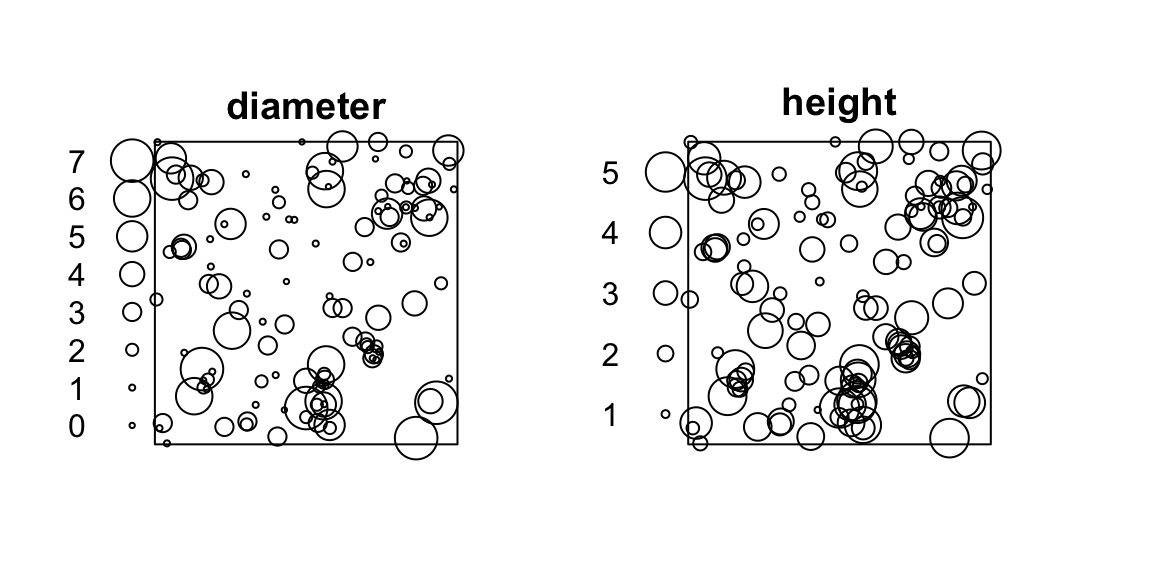
The point-pattern (ppp.object, Chapter 24) finpines from package spatstat.data (v3.1.9, GPL (>= 2)) has (Listing 9.38, Figure 9.7)
- 126 points;
- rectangle window;
- two numeric marks,
diameterandheight.
finpines
Code
par(mar = c(0,0,0,0))
spatstat.data::finpines |>
spatstat.geom::plot.ppp(main = '')finpines
finpines
spatstat.data::finpines |>
  spatstat.geom::print.ppp()
Marked planar point pattern: 126 points
Mark variables: diameter, height
window: rectangle = [-5, 5] x [-8, 2] metres9.12 flu
The hyper data frame (hyperframe, Chapter 16) flu from package spatstat.data (v3.1.9, GPL (>= 2)) has (Listing 9.39)
- 41 rows and 4 (hyper)columns (Listing 9.40)
- a point-pattern (
ppp, Chapter 24) hypercolumn$pattern - regular columns
$virustype,$stain,$frameid
flu
spatstat.data::flu |>
  spatstat.geom::print.hyperframe()
Hyperframe:
pattern virustype stain frameid
wt M2-M1 13 (ppp) wt M2-M1 13
wt M2-M1 22 (ppp) wt M2-M1 22
wt M2-M1 27 (ppp) wt M2-M1 27
wt M2-M1 43 (ppp) wt M2-M1 43
wt M2-M1 49 (ppp) wt M2-M1 49
wt M2-M1 65 (ppp) wt M2-M1 65
wt M2-M1 71 (ppp) wt M2-M1 71
wt M2-M1 84 (ppp) wt M2-M1 84
wt M2-HA 3 (ppp) wt M2-HA 3
wt M2-HA 4 (ppp) wt M2-HA 4
wt M2-HA 5 (ppp) wt M2-HA 5
wt M2-HA 17 (ppp) wt M2-HA 17
wt M2-HA 54 (ppp) wt M2-HA 54
wt M2-HA 74 (ppp) wt M2-HA 74
wt M2-HA 78 (ppp) wt M2-HA 78
wt M2-HA 82 (ppp) wt M2-HA 82
wt M2-HA 85 (ppp) wt M2-HA 85
wt M2-HA 100 (ppp) wt M2-HA 100
wt M2-HA 110 (ppp) wt M2-HA 110
mut1 M2-M1 11 (ppp) mut1 M2-M1 11
mut1 M2-M1 13 (ppp) mut1 M2-M1 13
mut1 M2-M1 15 (ppp) mut1 M2-M1 15
mut1 M2-M1 17 (ppp) mut1 M2-M1 17
mut1 M2-M1 28 (ppp) mut1 M2-M1 28
mut1 M2-M1 29 (ppp) mut1 M2-M1 29
mut1 M2-M1 33 (ppp) mut1 M2-M1 33
mut1 M2-M1 38 (ppp) mut1 M2-M1 38
mut1 M2-M1 41 (ppp) mut1 M2-M1 41
mut1 M2-M1 44 (ppp) mut1 M2-M1 44
mut1 M2-M1 59 (ppp) mut1 M2-M1 59
mut1 M2-HA 8 (ppp) mut1 M2-HA 8
mut1 M2-HA 14 (ppp) mut1 M2-HA 14
mut1 M2-HA 23 (ppp) mut1 M2-HA 23
mut1 M2-HA 42 (ppp) mut1 M2-HA 42
mut1 M2-HA 51 (ppp) mut1 M2-HA 51
mut1 M2-HA 59 (ppp) mut1 M2-HA 59
mut1 M2-HA 73 (ppp) mut1 M2-HA 73
mut1 M2-HA 79 (ppp) mut1 M2-HA 79
mut1 M2-HA 86 (ppp) mut1 M2-HA 86
mut1 M2-HA 104 (ppp) mut1 M2-HA 104
mut1 M2-HA 147 (ppp) mut1 M2-HA 147dimensions of flu
spatstat.data::flu |>
  spatstat.geom::dim.hyperframe()
[1] 41 49.13 gorillas
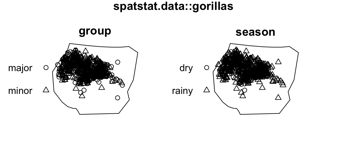
The point-pattern (ppp.object, Chapter 24) gorillas from package spatstat.data (v3.1.9, GPL (>= 2)) has (Listing 9.42, Figure 9.8)
- 647 points;
- polygonal window;
- two multi-type marks,
group(with two levels'major'and'minor') andseason(with two levels'dry'and'rainy').
gorillas
Code
par(mar = c(0,0,1,0))
spatstat.data::gorillas |>
spatstat.geom::plot.ppp(which.marks = c('group', 'season'))gorillas
gorillas
spatstat.data::gorillas |>
  spatstat.geom::print.ppp()
Marked planar point pattern: 647 points
Mark variables: group, season, date
window: polygonal boundary
enclosing rectangle: [580457.9, 585934] x [674172.8, 678739.2] metres9.14 gorillas.extra
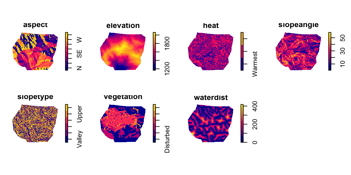
The pixel-image list (imlist, Chapter 19) gorillas.extra from package spatstat.data (v3.1.9, GPL (>= 2)) (Listing 9.44, Figure 9.9)
- inherits from the
S3class'solist'(Chapter 27, Listing 9.45); - contains 7 pixel-image (
im, Chapter 18) members (Listing 9.46).
gorillas.extra
Code
par(mar = c(0,0,0,0))
spatstat.data::gorillas.extra |>
plot(main = '')gorillas.extra
gorillas.extra
spatstat.data::gorillas.extraList of pixel images
aspect:
factor-valued pixel image
factor levels:
[1] "N" "NE" "E" "SE" "S" "SW" "W" "NW"
149 x 181 pixel array (ny, nx)
enclosing rectangle: [580440, 586000] x [674160, 678730] metres
elevation:
integer-valued pixel image
149 x 181 pixel array (ny, nx)
enclosing rectangle: [580440, 586000] x [674160, 678730] metres
heat:
factor-valued pixel image
factor levels:
[1] "Warmest" "Moderate" "Coolest"
149 x 181 pixel array (ny, nx)
enclosing rectangle: [580440, 586000] x [674160, 678730] metres
slopeangle:
real-valued pixel image
149 x 181 pixel array (ny, nx)
enclosing rectangle: [580440, 586000] x [674160, 678730] metres
slopetype:
factor-valued pixel image
factor levels:
[1] "Valley" "Toe" "Flat" "Midslope" "Upper" "Ridge"
149 x 181 pixel array (ny, nx)
enclosing rectangle: [580440, 586000] x [674160, 678730] metres
vegetation:
factor-valued pixel image
factor levels:
[1] "Disturbed" "Colonising" "Grassland" "Primary" "Secondary"
[6] "Transition"
149 x 181 pixel array (ny, nx)
enclosing rectangle: [580440, 586000] x [674160, 678730] metres
waterdist:
real-valued pixel image
149 x 181 pixel array (ny, nx)
enclosing rectangle: [580440, 586000] x [674160, 678730] metresgorillas.extra
spatstat.data::gorillas.extra |>
  class()
[1] "imlist" "solist" "anylist" "listof" "list" class of members of gorillas.extra
spatstat.data::gorillas.extra |>
  sapply(FUN = class)
aspect elevation heat slopeangle slopetype vegetation waterdist
"im" "im" "im" "im" "im" "im" "im" 9.15 hyytiala
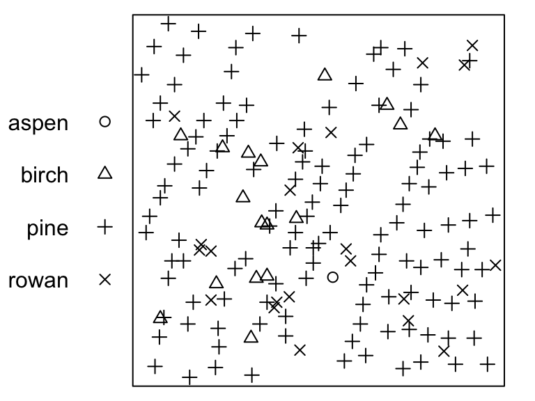
The point-pattern (ppp.object, Chapter 24) hyytiala from package spatstat.data (v3.1.9, GPL (>= 2)) has (Listing 9.48, Figure 9.10)
- 168 points;
- rectangle window;
- one multi-type mark with four levels,
'aspen','birch','pine'and'rowan'(Listing 9.49); 'vector'mark-format.
hyytiala
Code
par(mar = c(0,0,0,0))
spatstat.data::hyytiala |>
spatstat.geom::plot.ppp(main = NULL)hyytiala
hyytiala
spatstat.data::hyytiala |>
  spatstat.geom::print.ppp()
Marked planar point pattern: 168 points
Multitype, with levels = aspen, birch, pine, rowan
window: rectangle = [0, 20] x [0, 20] metreshyytiala
spatstat.data::hyytiala |>
  spatstat.geom::marks.ppp() |>
  table()
aspen birch  pine rowan
    1    17   128    22
9.16 Kovesi
The hyper data frame (hyperframe, Chapter 16) Kovesi from package spatstat.data (v3.1.9, GPL (>= 2)) has (Listing 9.50)
- 41 rows and 13 (hyper)columns (Listing 9.51)
- regular columns
$linear,$diverging, etc. - a
characterhypercolumn$values. This is alength-41 (Listing 9.53)anylist(Chapter 11, Listing 9.52) ofcharactervectors, each of them has a length of 256 (Listing 9.54).
Kovesi
spatstat.data::Kovesi |>
  spatstat.geom::print.hyperframe()
Hyperframe:
linear diverging rainbow cyclic isoluminant ternary colsig l1 l2 chro n
1 FALSE FALSE FALSE TRUE FALSE FALSE j 15 85 0 256
2 FALSE FALSE FALSE TRUE FALSE FALSE j 15 85 0 256
3 FALSE FALSE FALSE TRUE FALSE FALSE mrybm 35 75 68 256
4 FALSE FALSE FALSE TRUE FALSE FALSE mrybm 35 75 68 256
5 FALSE FALSE FALSE TRUE FALSE FALSE mygbm 30 95 78 256
6 FALSE FALSE FALSE TRUE FALSE FALSE mygbm 30 95 78 256
7 FALSE FALSE FALSE TRUE FALSE FALSE wrwbw 40 90 42 256
8 FALSE FALSE FALSE TRUE FALSE FALSE wrwbw 40 90 42 256
9 FALSE TRUE FALSE FALSE FALSE FALSE bkr 55 10 35 256
10 FALSE TRUE FALSE FALSE FALSE FALSE bky 60 10 30 256
11 FALSE TRUE FALSE FALSE FALSE FALSE bwr 40 95 42 256
12 FALSE TRUE FALSE FALSE FALSE FALSE bwr 55 98 37 256
13 FALSE TRUE FALSE FALSE FALSE FALSE cwm 80 100 22 256
14 FALSE TRUE FALSE FALSE FALSE FALSE gkr 60 10 40 256
15 FALSE TRUE FALSE FALSE FALSE FALSE gwr 55 95 38 256
16 FALSE TRUE FALSE FALSE FALSE FALSE gwv 55 95 39 256
17 FALSE TRUE FALSE FALSE TRUE FALSE cjm 75 75 24 256
18 FALSE TRUE FALSE FALSE TRUE FALSE cjo 70 70 25 256
19 TRUE TRUE FALSE FALSE FALSE FALSE bjr 30 55 53 256
20 TRUE TRUE FALSE FALSE FALSE FALSE bjy 30 90 45 256
21 FALSE TRUE TRUE FALSE FALSE FALSE bgymr 45 85 67 256
22 FALSE FALSE FALSE FALSE TRUE FALSE cgo 70 70 39 256
23 FALSE FALSE FALSE FALSE TRUE FALSE cgo 80 80 38 256
24 FALSE FALSE FALSE FALSE TRUE FALSE cm 70 70 39 256
25 TRUE FALSE FALSE FALSE FALSE FALSE b 5 95 73 256
26 TRUE FALSE FALSE FALSE FALSE FALSE b 95 50 20 256
27 TRUE FALSE FALSE FALSE FALSE FALSE bgy 10 95 74 256
28 TRUE FALSE FALSE FALSE FALSE FALSE bmw 5 95 89 256
29 TRUE FALSE FALSE FALSE FALSE FALSE bmy 10 95 78 256
30 TRUE FALSE FALSE FALSE FALSE FALSE g 5 95 69 256
31 TRUE FALSE FALSE FALSE FALSE FALSE gow 60 85 27 256
32 TRUE FALSE FALSE FALSE FALSE FALSE gow 65 90 35 256
33 TRUE FALSE FALSE FALSE FALSE FALSE j 0 100 0 256
34 TRUE FALSE FALSE FALSE FALSE FALSE j 10 95 0 256
35 TRUE FALSE FALSE FALSE FALSE FALSE kry 5 98 75 256
36 TRUE FALSE FALSE FALSE FALSE FALSE kryw 5 100 67 256
37 TRUE FALSE FALSE FALSE FALSE TRUE b 0 44 57 256
38 TRUE FALSE FALSE FALSE FALSE TRUE g 0 46 42 256
39 TRUE FALSE FALSE FALSE FALSE TRUE r 0 50 52 256
40 FALSE FALSE TRUE FALSE FALSE FALSE bgyr 35 85 73 256
41 FALSE FALSE TRUE FALSE FALSE FALSE bgyrm 35 85 71 256
cycsh values
1 0 (character)
2 25 (character)
3 0 (character)
4 25 (character)
5 0 (character)
6 25 (character)
7 0 (character)
8 25 (character)
9 0 (character)
10 0 (character)
11 0 (character)
12 0 (character)
13 0 (character)
14 0 (character)
15 0 (character)
16 0 (character)
17 0 (character)
18 0 (character)
19 0 (character)
20 0 (character)
21 0 (character)
22 0 (character)
23 0 (character)
24 0 (character)
25 0 (character)
26 0 (character)
27 0 (character)
28 0 (character)
29 0 (character)
30 0 (character)
31 0 (character)
32 0 (character)
33 0 (character)
34 0 (character)
35 0 (character)
36 0 (character)
37 0 (character)
38 0 (character)
39 0 (character)
40 0 (character)
41 0 (character)dimensions of Kovesi
spatstat.data::Kovesi |>
  spatstat.geom::dim.hyperframe()
[1] 41 13$values
spatstat.data::Kovesi$values |>
  class()
[1] "anylist" "listof" "list" $values
spatstat.data::Kovesi$values |>
  length()
[1] 41$values
spatstat.data::Kovesi$values |>
  lengths() |>
  unique.default()
[1] 2569.17 longleaf
The point-pattern (ppp.object, Chapter 24) longleaf from package spatstat.data (v3.1.9, GPL (>= 2)) has (Listing 9.56, Figure 9.11)
- 584 points;
- rectangle window;
- one numeric mark.
longleaf
Code
par(mar = c(0,0,0,0))
spatstat.data::longleaf |>
spatstat.geom::plot.ppp(main = NULL)longleaf
longleaf
spatstat.data::longleaf |>
  spatstat.geom::print.ppp()
Marked planar point pattern: 584 points
marks are numeric, of storage type 'double'
window: rectangle = [0, 200] x [0, 200] metres9.18 meningitis
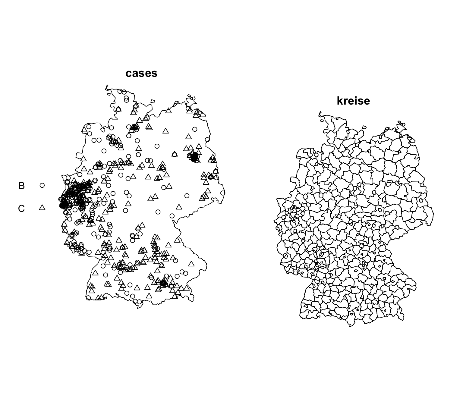
The spatial-object list (solist, Chapter 27) meningitis from package spatstat.data (v3.1.9, GPL (>= 2)) contains (Listing 9.58, Figure 9.12)
- a point-pattern (
ppp.object, Chapter 24)$cases; - a
tessellation (Chapter 29)$kreise.
meningitis
Code
par(mar = c(0,0,0,0))
spatstat.data::meningitis |>
spatstat.geom::plot.solist(main = '')meningitis
meningitis
spatstat.data::meningitisList of spatial objects
cases:
Marked planar point pattern: 636 points
Multitype, with levels = B, C
window: polygonal boundary
enclosing rectangle: [4031.295, 4672.253] x [2684.102, 3549.931] km
kreise:
Tessellation
Tiles are irregular polygons
413 tiles (irregular windows)
Tessellation has a data frame of marks:
$marks: double
window: polygonal boundary
enclosing rectangle: [4031.295, 4672.253] x [2684.102, 3549.931] km9.19 nbfires
The point-pattern (ppp.object, Chapter 24) nbfires from package spatstat.data (v3.1.9, GPL (>= 2)) has (Listing 9.60, Figure 9.13)
- 7108 points;
- polygonal window;
- multi-type marks, e.g.,
$fire.type,$causeand$ign.src; - numeric marks, e.g.,
$fnl.size.
nbfires
Code
par(mar = c(0,0,1,0))
spatstat.data::nbfires |>
  spatstat.geom::plot.ppp(which.marks = c('fire.type', 'cause', 'ign.src', 'fnl.size'))
Warning: Only 10 out of 16 symbols are shown in the symbol mapnbfires
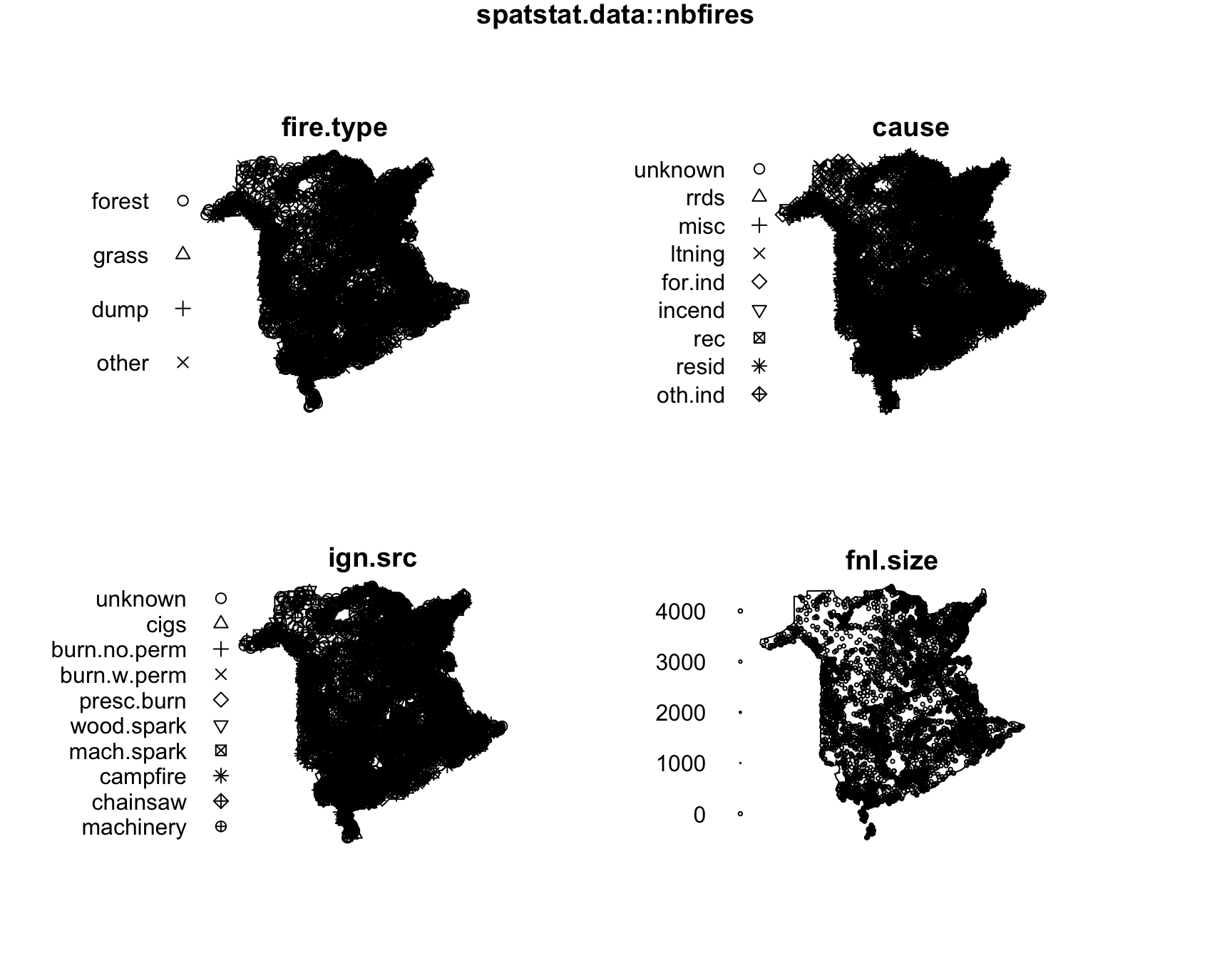
nbfires
spatstat.data::nbfires |>
  spatstat.geom::print.ppp()
Warning: some mark values are NA in the point pattern xMarked planar point pattern: 7108 points
Mark variables:
year fire.type dis.date dis.julian out.date out.julian cause ign.src
fnl.size
window: polygonal boundary
enclosing rectangle: [0, 1000] x [0, 958.9142] units (one unit = 0.403716 km)9.20 osteo
The hyper data frame (hyperframe, Chapter 16) osteo from package spatstat.data (v3.1.9, GPL (>= 2)) has (Listing 9.61)
- 40 rows and 5 (hyper)columns (Listing 9.62)
- the serial number of sampling volume
$bricknested in the bone sample$id - a three-dimensional point-pattern (
pp3, Chapter 23) hypercolumn$pts
osteo
spatstat.data::osteo |>
  spatstat.geom::print.hyperframe()
Hyperframe:
id shortid brick pts depth
1 c77za4 4 1 (pp3) 45
2 c77za4 4 2 (pp3) 60
3 c77za4 4 3 (pp3) 55
4 c77za4 4 4 (pp3) 60
5 c77za4 4 5 (pp3) 85
6 c77za4 4 6 (pp3) 90
7 c77za4 4 7 (pp3) 95
8 c77za4 4 8 (pp3) 65
9 c77za4 4 9 (pp3) 100
10 c77za4 4 10 (pp3) 100
11 c77za5 5 1 (pp3) 45
21 c77za5 5 2 (pp3) 30
31 c77za5 5 3 (pp3) 40
41 c77za5 5 4 (pp3) 45
51 c77za5 5 5 (pp3) 40
61 c77za5 5 6 (pp3) 50
71 c77za5 5 7 (pp3) 40
81 c77za5 5 8 (pp3) 60
91 c77za5 5 9 (pp3) 65
101 c77za5 5 10 (pp3) 60
12 c77za8 8 1 (pp3) 40
22 c77za8 8 2 (pp3) 55
32 c77za8 8 3 (pp3) 60
42 c77za8 8 4 (pp3) 50
52 c77za8 8 5 (pp3) 45
62 c77za8 8 6 (pp3) 30
72 c77za8 8 7 (pp3) 50
82 c77za8 8 8 (pp3) 45
92 c77za8 8 9 (pp3) 70
102 c77za8 8 10 (pp3) 110
13 c77za9 9 1 (pp3) 60
23 c77za9 9 2 (pp3) 65
33 c77za9 9 3 (pp3) 55
43 c77za9 9 4 (pp3) 70
53 c77za9 9 5 (pp3) 55
63 c77za9 9 6 (pp3) 100
73 c77za9 9 7 (pp3) 80
83 c77za9 9 8 (pp3) 75
93 c77za9 9 9 (pp3) 85
103 c77za9 9 10 (pp3) 60dimensions of osteo
spatstat.data::osteo |>
  spatstat.geom::dim.hyperframe()
[1] 40 59.21 spruces
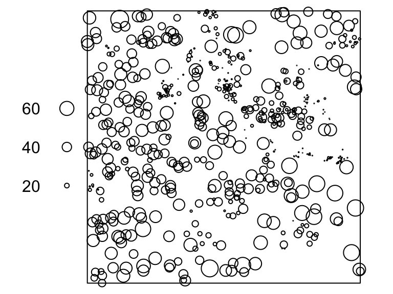
The point-pattern (ppp.object, Chapter 24) spruces from package spatstat.data (v3.1.9, GPL (>= 2)) has (Listing 9.64, Figure 9.14)
- 134 points;
- rectangle window;
- one numeric mark.
spruces
Code
par(mar = c(0,0,0,0))
spatstat.data::spruces |>
spatstat.geom::plot.ppp(main = NULL)spruces
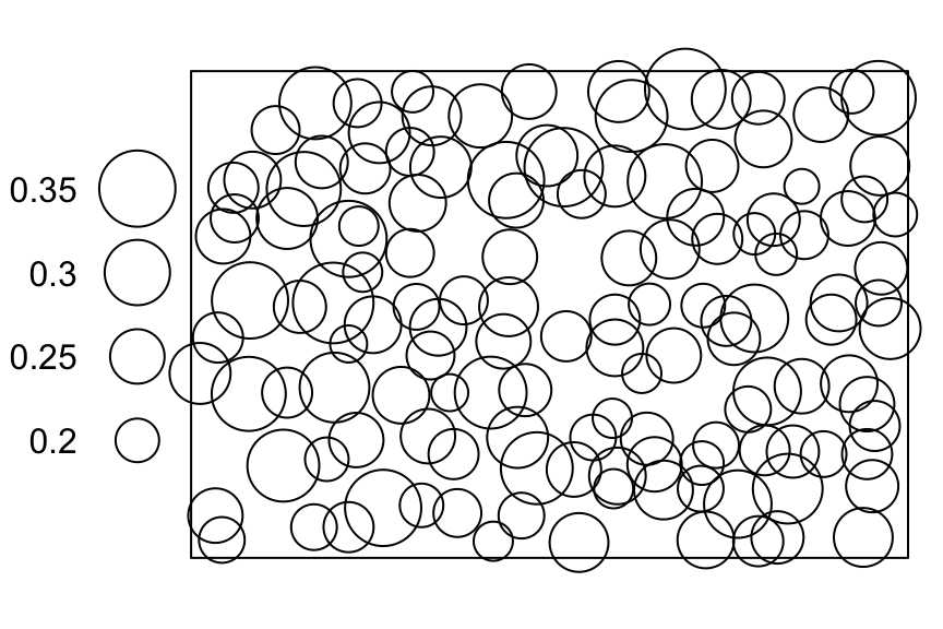
spruces
spatstat.data::spruces |>
  spatstat.geom::print.ppp()
Marked planar point pattern: 134 points
marks are numeric, of storage type 'double'
window: rectangle = [0, 56] x [0, 38] metres9.22 swedishpines
The point-pattern (ppp.object, Chapter 24) swedishpines from package spatstat.data (v3.1.9, GPL (>= 2)) has (Listing 9.66, Figure 9.15)
- the \(x\)- and \(y\)-coordinates of 71 points;
- rectangle window;
- no marks, i.e.,
'none'mark-format.
swedishpines
Code
par(mar = c(0,0,0,0))
spatstat.data::swedishpines |>
spatstat.geom::plot.ppp(main = NULL)swedishpines
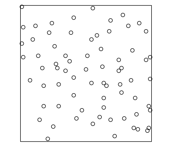
swedishpines
spatstat.data::swedishpines |>
  spatstat.geom::print.ppp()
Planar point pattern: 71 points
window: rectangle = [0, 96] x [0, 100] units (one unit = 0.1 metres)9.23 VADeaths
The matrix VADeaths from package datasets (R version 4.5.3 (2026-03-11)) has (Listing 9.67)
- 5 rows and 4 columns (Listing 9.68)
VADeaths
datasets::VADeaths |>
  print.default()
Rural Male Rural Female Urban Male Urban Female
50-54 11.7 8.7 15.4 8.4
55-59 18.1 11.7 24.3 13.6
60-64 26.9 20.3 37.0 19.3
65-69 41.0 30.9 54.6 35.1
70-74 66.0 54.3 71.1 50.0dimensions of VADeaths
datasets::VADeaths |>
  dim()
[1] 5 49.24 vesicles
The point-pattern (ppp.object, Chapter 24) vesicles from package spatstat.data (v3.1.9, GPL (>= 2)) has (Listing 9.70, Figure 9.16)
- the \(x\)- and \(y\)-coordinates of 37 points;
- polygonal window;
- no marks, i.e.,
'none'mark-format.
vesicles
Code
par(mar = c(0,0,0,0))
spatstat.data::vesicles |>
spatstat.geom::plot.ppp(main = NULL)vesicles
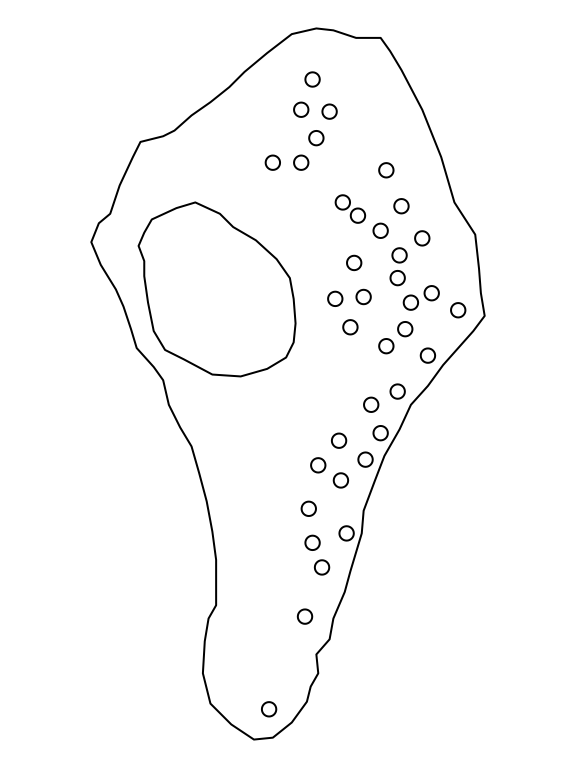
vesicles
spatstat.data::vesicles |>
  spatstat.geom::print.ppp()
Planar point pattern: 37 points
window: polygonal boundary
enclosing rectangle: [22.6796, 586.2292] x [11.9756, 1030.7] nm9.25 vesicles.extra
The spatial-object list (solist, Chapter 27) vesicles.extra from package spatstat.data (v3.1.9, GPL (>= 2)) has (Listing 9.71, Listing 9.72)
- a line-segment-pattern (
psp, Chapter 26)$activezone - three windows:
$mitochondria,$presynapseand$mask
vesicles.extra
spatstat.data::vesicles.extraList of spatial objects
activezone:
planar line segment pattern: 9 line segments
window: rectangle = [0, 625] x [0, 1050] nm
mitochondria:
window: polygonal boundary
enclosing rectangle: [90.41389, 315.29187] x [532.1753, 781.4376] nm
presynapse:
window: polygonal boundary
enclosing rectangle: [22.6796, 586.2292] x [11.9756, 1030.7] nm
mask:
window: binary image mask
420 x 250 pixel array (ny, nx)
enclosing rectangle: [0, 250] x [0, 420] unitsclass of members of vesicles.extra
spatstat.data::vesicles.extra |>
  lapply(FUN = class)
$activezone
[1] "psp" "list"
$mitochondria
[1] "owin"
$presynapse
[1] "owin"
$mask
[1] "owin"9.26 waterstriders
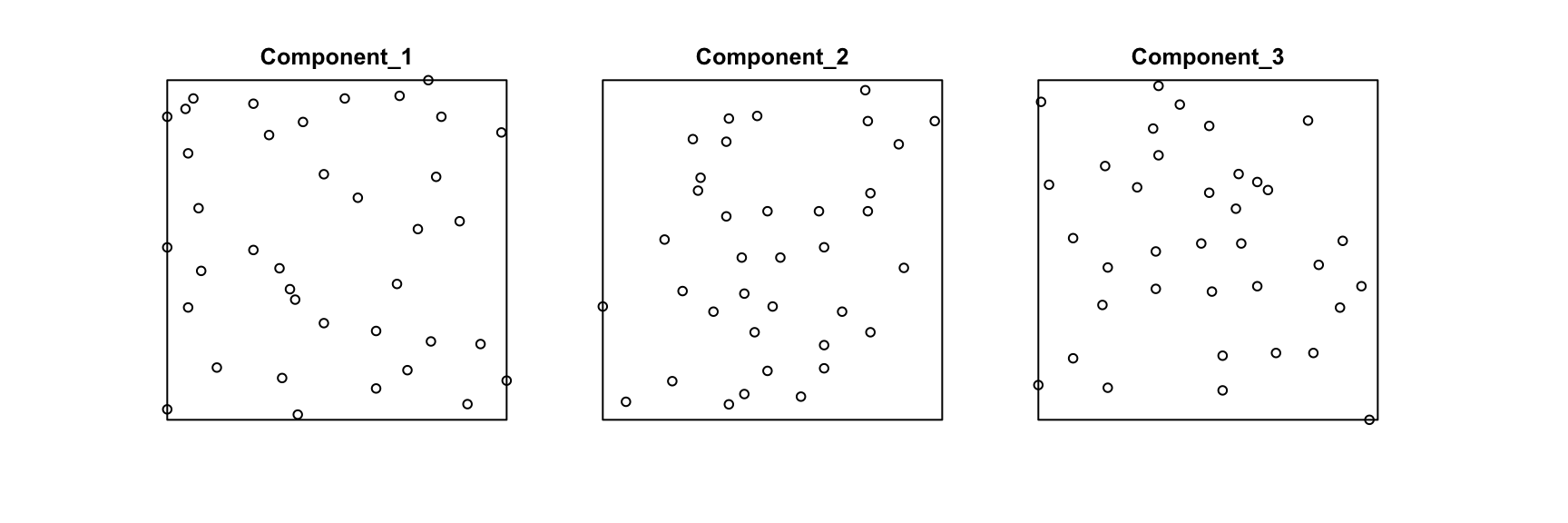
The point-pattern-list (ppplist, Chapter 25) waterstriders from package spatstat.data (v3.1.9, GPL (>= 2)) (Listing 9.74, Figure 9.17)
- inherits from the
S3class'solist'(Chapter 27) - contains 3 point-pattern (
ppp.object, Chapter 24) members (Listing 9.75).
waterstriders
Code
par(mar = c(0,0,0,0))
spatstat.data::waterstriders |>
spatstat.geom::plot.solist(main = '')waterstriders
waterstriders
spatstat.data::waterstridersList of point patterns
Component 1:
Planar point pattern: 38 points
window: rectangle = [0, 48.1] x [0, 48.1] cm
Component 2:
Planar point pattern: 36 points
window: rectangle = [0, 48.8] x [0, 48.8] cm
Component 3:
Planar point pattern: 36 points
window: rectangle = [0, 46.4] x [0, 46.4] cmclass of members of waterstriders
spatstat.data::waterstriders |>
  sapply(FUN = class)
[1] "ppp" "ppp" "ppp"