4 Simulation
These packages (Note 1) are a one-person project undergoing rapid evolution. Backward compatibility (per Hadley Wickham) is provided as a courtesy rather than a guarantee.
Until further notice, these packages should
- not be used as the basis for research grant applications or referenced in final research progress reports,
- not be cited as an actively maintained tool in a peer-reviewed manuscript,
- not be used to support or fulfill requirements for pursuing an academic degree.
In addition, work primarily based on these packages (Note 1) should not be presented at academic conferences or similar scholarly venues.
Furthermore, a person’s ability to use these packages (Note 1) does not necessarily imply an understanding of their underlying mechanisms. Accordingly, demonstration of their use alone should not be considered sufficient evidence of expertise, nor should it be credited as a basis for academic promotion or advancement.
These statements do not apply to the contributors (Tip 1) to these packages (Note 1) with respect to their specific contributions.
These statements do not apply when the maintainer of these packages (Note 1), Tingting Zhan, is credited as the first author, the lead author, and/or the corresponding author in a peer-reviewed manuscript, or as the Principal Investigator or Co-Principal Investigator in a research grant application and/or a final research progress report.
These statements are advisory in nature and do not modify or restrict the rights granted under the GNU General Public License https://www.r-project.org/Licenses/.
The examples in Chapter 4 require
library(groupedHyperframe.random)4.1 Simulated Point-Pattern
The function .rppp() (Chapter 36) simulates superimposed point-patterns (ppp.object, Chapter 24) via vectorized parameterization, which is supported in the parameter-specification of both the random point-pattern and the random marks.
Listing 4.1 simulates an \(x\)- and \(y\)-coordinates only, two superimposed Matérn (1986)’s cluster processes \((\kappa, \mu, s)\) with parameters \((\kappa_1, \mu_1, s_1) = (10,8,.15)\) and \((\kappa_2, \mu_2, s_2) = (5,4,.06)\) using a vectorized parameterization of Table 4.1.
kappa \(\kappa\) |
mu \(\mu\) |
scale \(s\) |
|
|---|---|---|---|
| Vecterization | \((\kappa_1, \kappa_2)\) | \((\mu_1, \mu_2)\) | \((s_1, s_2)\) |
| Restriction | \(\kappa_i>1\) | \(\mu_i>1\) | \(s_i>0\) |
set.seed(12); r = .rppp(rMatClust(kappa = c(10, 5), mu = c(8, 4), scale = c(.15, .06)))Point-pattern simulated by `spatstat.random::rMatClust()`Listing 4.2 simulates two superimposed marked point-patterns,
- one marked point-pattern with
- \(x\)- and \(y\)-coordinates by Matérn (1986)’s cluster process with parameters \((\kappa_1,\mu_1,s_1) = (10,8,.15)\);
- log-normal \((\log\mu, \log\sigma)\) marks with parameters \((\log\mu_1,\log\sigma_1)=(3,.4)\);
- negative-binomial \((r, p)\) marks with parameters \((r,p)=(4,.3)\).
- another marked point-pattern with
- \(x\)- and \(y\)-coordinates by Matérn (1986)’s cluster process with parameters \((\kappa_2,\mu_2,s_2) = (5,4,.06)\);
- log-normal marks with parameters \((\log\mu_2,\log\sigma_2)=(5,.2)\)
- negative-binomial marks with parameters \((r,p)=(4,.3)\).
using a vectorized parameterization of Table 4.2.
kappa \(\kappa\) |
mu \(\mu\) |
scale \(s\) |
meanlog \(\log\mu\) |
sdlog \(\log\sigma\) |
size \(r\) |
prob \(p\) |
|
|---|---|---|---|---|---|---|---|
| Vec. | \((\kappa_1, \kappa_2)\) | \((\mu_1, \mu_2)\) | \((s_1, s_2)\) | \((\log\mu_1, \log\mu_2)\) | \((\log\sigma_1, \log\sigma_2)\) | \((r_1, r_2)\) | \((p_1, p_2)\) |
| Res. | \(\kappa_i>1\) | \(\mu_i>1\) | \(s_i>0\) | (none) | \(\log\sigma_i>0\) | \(r_i>0\) | \(0<p_i<1\) |
set.seed(25); r1 = .rppp(
  rMatClust(kappa = c(10, 5), mu = c(8, 4), scale = c(.15, .06)),
  rlnorm(meanlog = c(3, 5), sdlog = c(.4, .2)),
  rnbinom(size = 4, prob = .3) # shorter arguments recycled
)
Point-pattern simulated by `spatstat.random::rMatClust()`Mark simulated by `stats::rlnorm()`
Mark simulated by `stats::rnbinom()`Listing 4.3 simulates two superimposed point-patterns,
- one marked point-pattern with
- \(x\)- and \(y\)-coordinates by Poisson point-pattern \(\lambda\) with parameter \(\lambda_1=3\),
- log-normal marks with parameters \((\log\mu_1,\log\sigma_1)=(3,.4)\);
- negative-binomial marks with parameters \((r_1,p_1)=(4,.3)\).
- another marked point-pattern with
- \(x\)- and \(y\)-coordinates by Poisson point-pattern with parameters \(\lambda_2=6\)
- log-normal marks with parameters \((\log\mu_2,\log\sigma_2)=(5,.2)\)
- negative-binomial marks with parameters \((r_2,p_2)=(6,.1)\).
using a vectorized parameterization of Table 4.3.
lambda \(\lambda\) |
meanlog \(\log\mu\) |
sdlog \(\log\sigma\) |
size \(r\) |
prob \(p\) |
|
|---|---|---|---|---|---|
| Vecterization | \((\lambda_1, \lambda_2)\) | \((\log\mu_1, \log\mu_2)\) | \((\log\sigma_1, \log\sigma_2)\) | \((r_1, r_2)\) | \((p_1, p_2)\) |
| Restriction | \(\lambda_i>0\) | (none) | \(\log\sigma_i>0\) | \(r_i>0\) | \(0<p_i<1\) |
set.seed(62); r2 = .rppp(
  rpoispp(lambda = c(3, 6)),
  rlnorm(meanlog = c(3, 5), sdlog = c(.4, .2)),
  rnbinom(size = c(4, 6), prob = c(.3, .1))
)
Point-pattern simulated by `spatstat.random::rpoispp()`Mark simulated by `stats::rlnorm()`
Mark simulated by `stats::rnbinom()`Listing 4.4 superimposes the simulated (marked) point-patterns r1 and r2 (Listing 4.2, Listing 4.3).
spatstat.geom::superimpose.ppp(r1, r2)Marked planar point pattern: 140 points
Mark variables: rlnorm, rnbinom
window: rectangle = [0, 1] x [0, 1] units4.2 Simulated Grouped Hyper Data Frame
The function grouped_rppp() (Chapter 32) simulates a grouped hyper data frame containing one-and-only-one point-pattern (ppp) hypercolumn (Chapter 3) via matrix parameterization, which is supported in the subject-specific parameter-specification of both the random point-pattern and the random marks.
4.2.1 with Superimposed Matérn (1986)’s Cluster Processes
Table 4.4 outlines the three steps described in Section 4.2.1,
| To Simulate | Primary Function | |
|---|---|---|
| 1. | subject-specific parameters of (marked) point-patterns, based on multivariate normal distribution, Listing 4.5 | mvrnorm2() (Chapter 33) |
| 2. | number of (marked) point-patterns per subject, Listing 4.7 | sample() |
| 3. | grouped hyper data frame with one-and-only-one ppp-hypercolumn, Listing 4.8 |
grouped_rppp() (Chapter 32) |
Consider two superimposed Matérn (1986)’s cluster processes, each with one log-normal mark. The population parameters are
- \(x\)- and \(y\)-coordinates by Matérn (1986)’s cluster process \((\kappa_1,\mu_1,s_1) = (3,10,.4)\), with a log-normal mark \((\log\mu_1,\log\sigma_1)=(3,.4)\)
- \(x\)- and \(y\)-coordinates by Matérn (1986)’s cluster process \((\kappa_2,\mu_2,s_2) = (2,5,.2)\), with a log-normal mark \((\log\mu_2,\log\sigma_2)=(5,.2)\)
Listing 4.5 simulates for three (3L) subjects (e.g., patients). The subject-specific parameters deviate from the population parameters under a multivariate normal distribution specified by the standard deviation(s) \(\sigma\) of the subject-specific random effects, i.e., \(\sigma_\kappa=.2\), \(\sigma_\mu=.5\), \(\sigma_s=.05\), \(\sigma_{\log\mu}=.1\) and \(\sigma_{\log\sigma}=.01\), as well as the restrictions in Table 4.2.
p_Matern
set.seed(39); p_Matern = mapply(
  FUN = mvrnorm2,
  mu = list(kappa = c(3,2), mu = c(10,5), scale = c(.4,.2), meanlog = c(3,5), sdlog = c(.4,.2)),
  sd = list(kappa = .2, mu = .5, scale = .05, meanlog = .1, sdlog = .01),
  MoreArgs = list(n = 3L, row.prefix = 'Subj', col.prefix = 'Pattern'),
  SIMPLIFY = FALSE
) |>
  within.list(expr = {
    kappa = pmax(kappa, 1 + .Machine$double.eps)
    mu = pmax(mu, 1 + .Machine$double.eps)
    scale = pmax(scale, .Machine$double.eps)
    sdlog = pmax(sdlog, .Machine$double.eps)
  })
Listing 4.6 shows the subject-specific parameters p_Matern as a list of matrices, where each matrix represents one parameter used in generating the random marked point-patterns. In these matrices,
- Each row corresponds to a subject; i.e., each matrix in
p_Materncontains three (3L) rows, one for each of the three (3L) subjects; - Each column corresponds to a random generation parameter for each superimposed marked point-pattern; i.e., each matrix in
p_Materncontains two (2L) columns, one for each of the two (2L) marked Matérn (1986)’s cluster processes to be superimposed.
p_Matern (Listing 4.5)
p_Matern$kappa
Pattern 1 Pattern 2
Subj 1 3.119196 1.962887
Subj 2 2.906535 1.754151
Subj 3 2.915672 1.914559
$mu
Pattern 1 Pattern 2
Subj 1 9.519187 4.489174
Subj 2 9.947885 4.688761
Subj 3 10.029897 5.418501
$scale
Pattern 1 Pattern 2
Subj 1 0.4227306 0.2351866
Subj 2 0.4058303 0.1622515
Subj 3 0.3726093 0.1727232
$meanlog
Pattern 1 Pattern 2
Subj 1 2.982251 5.007964
Subj 2 2.878996 4.976754
Subj 3 3.034019 4.852771
$sdlog
Pattern 1 Pattern 2
Subj 1 0.4055664 0.1975062
Subj 2 0.4172841 0.2115214
Subj 3 0.4076479 0.1970090Listing 4.7 simulates one (1L) to four (4L) point-patterns (e.g., medical images) for each of the three (3L) subjects (e.g., patients).
set.seed(37); (n = sample(x = 1:4, size = 3L, replace = TRUE)) [1] 2 3 4Listing 4.8 simulates a grouped hyper data frame with
- one point-pattern (
ppp) hypercolumn, based on the subject-specific parameters in each matrix ofp_Matern(Listing 4.6); and - one-or-more regular columns representing the grouping structure.
r_Matern (Listing 4.5, Listing 4.7)
set.seed(76); r_Matern = p_Matern |>
  with.default(expr = {
    grouped_rppp(
      rMatClust(kappa = kappa, scale = scale, mu = mu),
      rlnorm(meanlog = meanlog, sdlog = sdlog),
      n = n
    )
  })
r_Matern
Grouped Hyper Data Frame: ~g1
3 g1
ppp g1 g2
1 (ppp) 1 1
2 (ppp) 1 2
3 (ppp) 2 1
4 (ppp) 2 2
5 (ppp) 2 3
6 (ppp) 3 1
7 (ppp) 3 2
8 (ppp) 3 3
9 (ppp) 3 44.2.2 with Superimposed Poisson Point-Pattern
Table 4.5 outlines the three steps described in Section 4.2.2,
| To Simulate | Primary Function | |
|---|---|---|
| 1. | subject-specific parameters of (marked) point-patterns, based on multivariate normal distribution, Listing 4.9 | mvrnorm2() (Chapter 33) |
| 2. | number of (marked) point-patterns per subject, Listing 4.7 | sample() |
| 3. | grouped hyper data frame with one-and-only-one ppp-hypercolumn, Listing 4.11 |
grouped_rppp() (Chapter 32) |
Consider two superimposed Poisson point-pattern, each with one negative-binomial mark. The population parameters are
- \(x\)- and \(y\)-
coordsby Poisson point-pattern \(\lambda_1=3\), with a negative-binomial mark \((r_1,p_1)=(4,.3)\). - \(x\)- and \(y\)-
coordsby Poisson point-pattern \(\lambda_2=6\), with a negative-binomial mark \((r_2,p_2)=(6,.1)\).
Listing 4.9 also simulate for three (3L) subjects (e.g., patients). The subject-specific parameters deviate from the population parameters under a multivariate normal distribution specified by the standard deviation(s) \(\sigma\) of the subject-specific random effects, i.e., \(\sigma_\lambda=.1\), \(\sigma_r=.2\) and \(\sigma_p=.05\), as well as the restrictions of Table 4.3.
p_Poisson
set.seed(39); p_Poisson = mapply(
  FUN = mvrnorm2,
  mu = list(lambda = c(3, 6), size = c(4, 6), prob = c(.3, .1)),
  sd = list(lambda = .1, size = .2, prob = .05),
  MoreArgs = list(n = 3L, row.prefix = 'Subj', col.prefix = 'Pattern'),
  SIMPLIFY = FALSE
) |>
  within.list(expr = {
    lambda = pmax(lambda, .Machine$double.eps)
    size = pmax(size, .Machine$double.eps)
    prob = pmin(pmax(prob, .Machine$double.eps), 1 - .Machine$double.eps)
})p_Poisson (Listing 4.9)
p_Poisson$lambda
Pattern 1 Pattern 2
Subj 1 3.059598 5.981443
Subj 2 2.953268 5.877076
Subj 3 2.957836 5.957280
$size
Pattern 1 Pattern 2
Subj 1 3.807675 5.795670
Subj 2 3.979154 5.875505
Subj 3 4.011959 6.167400
$prob
Pattern 1 Pattern 2
Subj 1 0.3227306 0.13518657
Subj 2 0.3058303 0.06225150
Subj 3 0.2726093 0.07272321Listing 4.11 simulates a grouped hyper data frame using the same grouping size as in Listing 4.7.
r_Poisson (Listing 4.9, Listing 4.7)
set.seed(76); r_Poisson = p_Poisson |>
  with.default(expr = {
    grouped_rppp(
      rpoispp(lambda = lambda),
      rnbinom(size = size, prob = prob),
      n = n
    )
  })
r_Poisson
Grouped Hyper Data Frame: ~g1
3 g1
ppp g1 g2
1 (ppp) 1 1
2 (ppp) 1 2
3 (ppp) 2 1
4 (ppp) 2 2
5 (ppp) 2 3
6 (ppp) 3 1
7 (ppp) 3 2
8 (ppp) 3 3
9 (ppp) 3 44.2.3 Superimpose Grouped Hyper Data Frames
Listing 4.12 superimposes the simulated grouped hyper data frames r_Matern and r_Poisson (Listing 4.8, Listing 4.11),
(r = spatstat.geom::superimpose(r_Matern, r_Poisson))Grouped Hyper Data Frame: ~g1
3 g1
ppp g1 g2
1 (ppp) 1 1
2 (ppp) 1 2
3 (ppp) 2 1
4 (ppp) 2 2
5 (ppp) 2 3
6 (ppp) 3 1
7 (ppp) 3 2
8 (ppp) 3 3
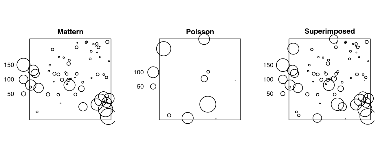
9 (ppp) 3 4Listing 4.13 checks the return of superimposing (Listing 4.12). Note that the marks may be plotted on different scales.
par(mar = c(0,0,0,0))
z = list(
  Mattern = r_Matern$ppp,
  Poisson = r_Poisson$ppp,
  Superimposed = r$ppp
) |>
  .mapply(FUN = spatstat.geom::solist, dots = _, MoreArgs = NULL) |>
  do.call(what = spatstat.geom::anylist, args = _)
z[[7L]] |>
  spatstat.geom::plot.solist(main = '')