The S3 generic function spatstat.explore::as.fv() (v3.7.0.4) converts R objects of various classes into a function-value-table. Listing 19.1 summarizes the S3 methods for the generic function as.fv() in the spatstat.* family of packages,
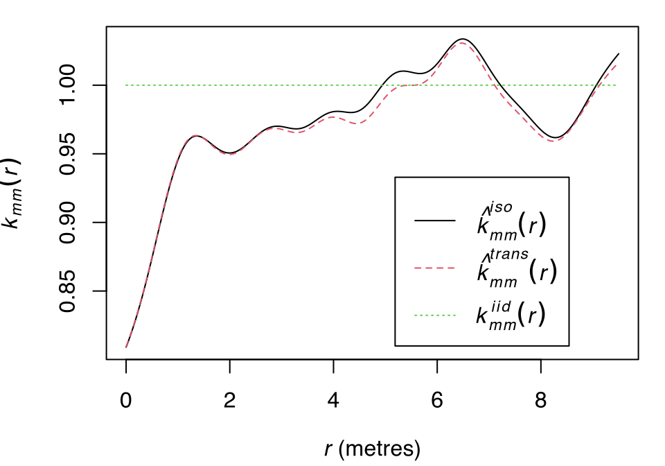
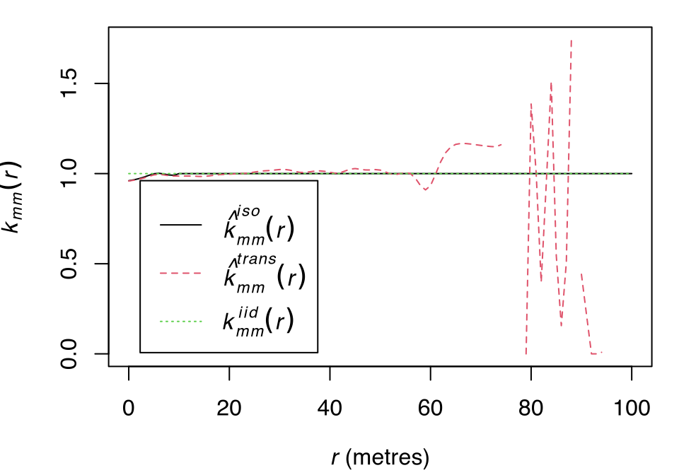
spruces_k |> spatstat.explore::print.fv()# Function value object (class 'fv')# for the function r -> k[mm](r)# ................................................................................# Math.label Description # r r distance argument r # theo {k[mm]^{iid}}(r) theoretical value (independent marks) for k[mm](r)# trans {hat(k)[mm]^{trans}}(r) translation-corrected estimate of k[mm](r) # iso {hat(k)[mm]^{iso}}(r) Ripley isotropic correction estimate of k[mm](r) # ................................................................................# Default plot formula: .~r# where "." stands for 'iso', 'trans', 'theo'# Recommended range of argument r: [0, 9.5]# Available range of argument r: [0, 9.5]# Unit of length: 1 metre
The S3 generic function keyval(), for key value, finds various function values (default being the recommended) in a function-value-table, or an R object containing one or more function-value-tables. The term “key” comes from the invisible return of the S3 method spatstat.explore::plot.fv() (v3.7.0.4) (Listing 19.7). Package groupedHyperframe (v0.3.4) implements the following S3 methods (Table 19.3),
Table 19.3: S3 methods of groupedHyperframe::keyval (v0.3.4)
visible
isS4
keyval.fv
TRUE
FALSE
keyval.fvlist
TRUE
FALSE
keyval.hyperframe
TRUE
FALSE
Listing 19.7: Review: the invisible return of function plot.fv()
The S3 method keyval.fv() finds various function values (default being the recommended) in a function-value-table, with the corresponding function argument as the vector names.
Listing 19.8 finds the recommended function value in the function-value-table spruces_k (Listing 19.3).
Listing 19.8: Example: function keyval.fv() (Listing 19.3)
The S3 method spatstat.explore::with.fv() (v3.7.0.4) is capable of creating identical returns as the S3 method keyval.fv() (Listing 19.10, Listing 19.11). The internal utility function getValues() defined in the local environment of the S3 group-generic-method Summary.fv() (Listing 19.12) vectorizes all function values. Table 19.4 explains their differences and connections.
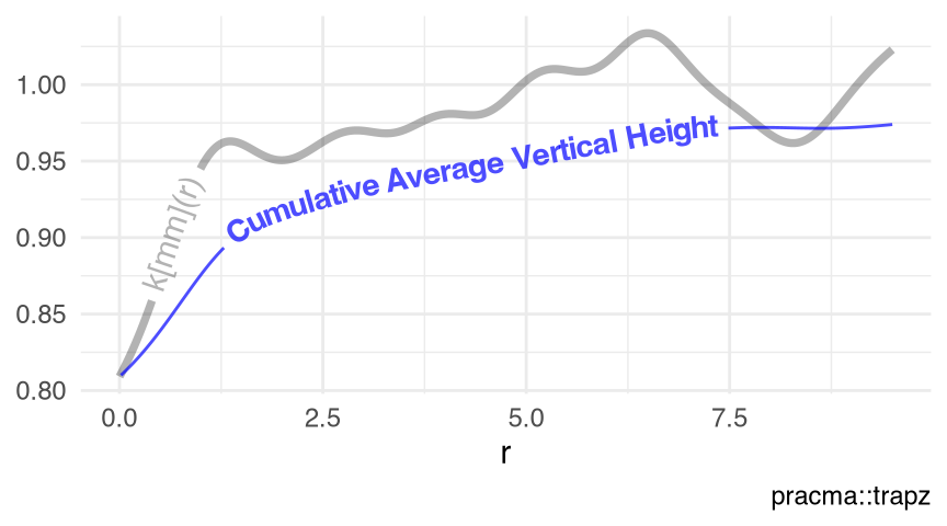
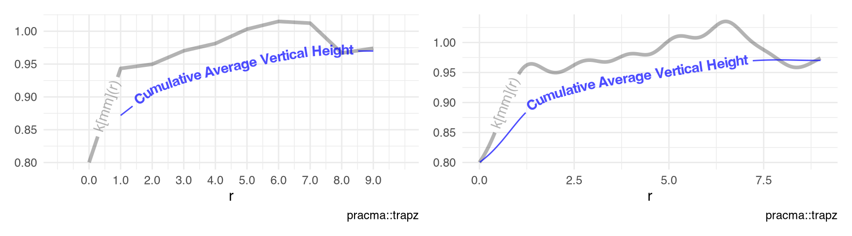
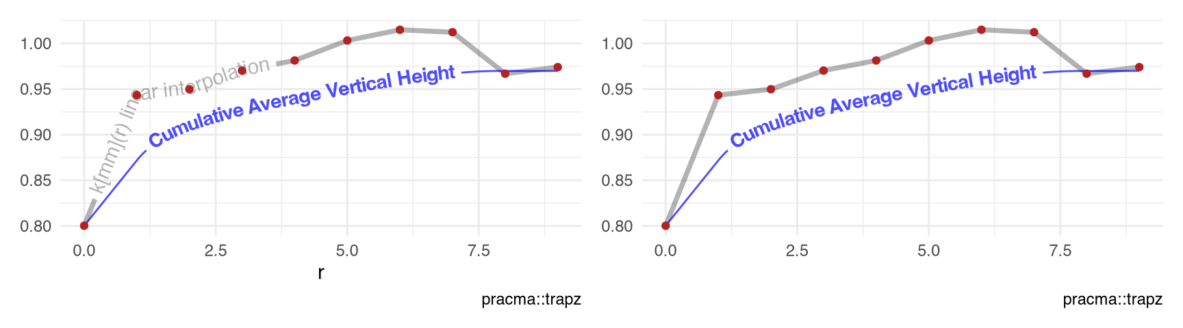
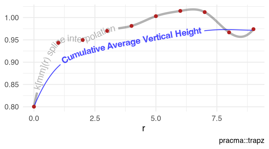
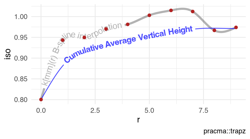
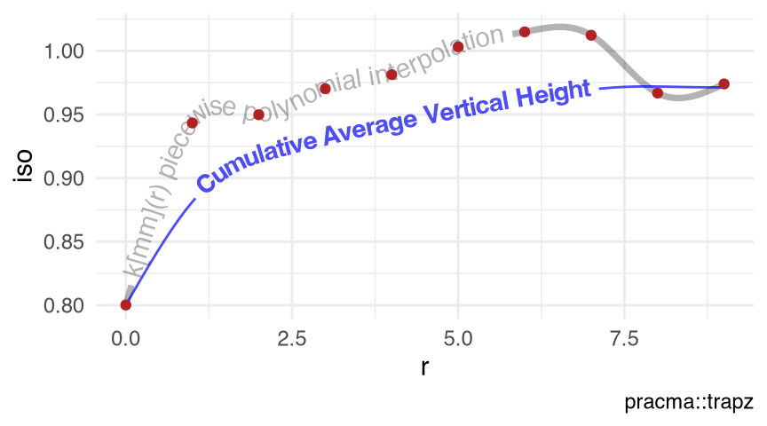
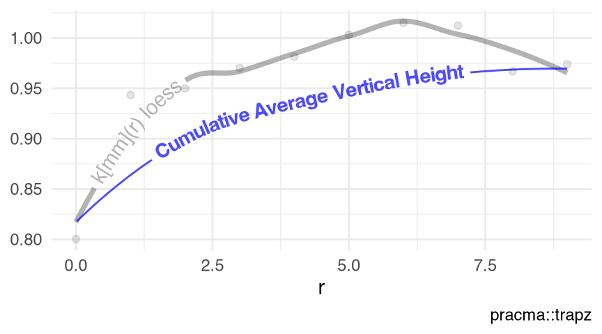
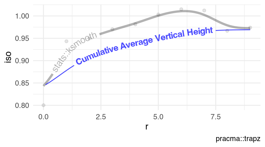
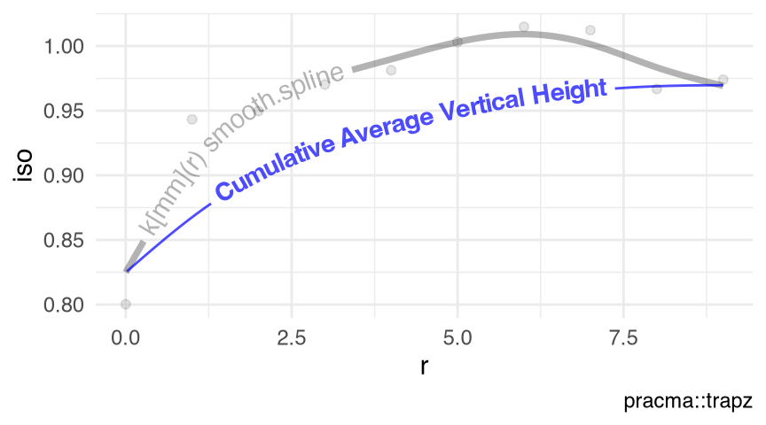
19.3 Cumulative Average Vertical Height of Trapzoidal Integration
The S3 method cumvtrapz.fv() (Section 10.2, Table 10.1) calculates the cumulative average vertical height of the trapezoidal integration (Section 10.2) under the recommended function values.
The S3 method visualize_vtrapz.fv() (Section 10.3, Table 10.2) visualizes the cumulative average vertical height of the trapezoidal integration (Section 10.2) under the recommended function values
Figure 19.2: Cumulative Average Vertical Height of the Trapezoidal Integration (Section 10.2) of spruces_k (Listing 19.3)
19.4\(r_\text{max}\)
The S3 method .rmax.fv() (Section 35.10, Table 35.13), often used as an internal utility function, simply grabs the maximum value of the \(r\)-vector in a function-value-table.
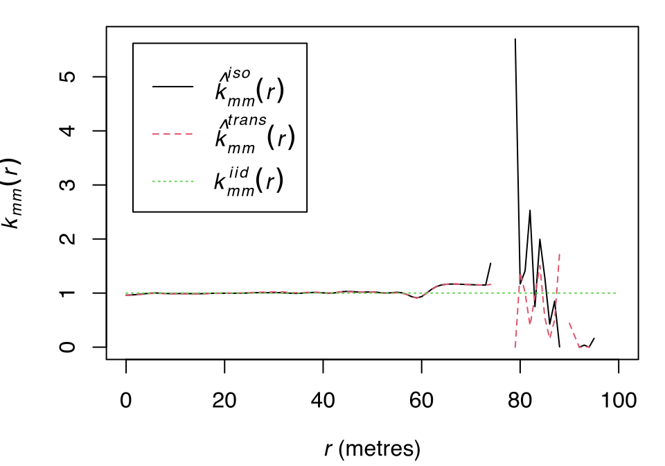
Function spatstat.explore::markcorr() is the workhorse inside the functions Emark(), Vmark() and markvario() (v3.7.0.4). Function markcorr() provides a default argument of parameter \(r\)-vector (Section 35.10), at which the mark correlation function \(k_f(r)\) are evaluated. Function markcorr() relies on the un-exported workhorse function spatstat.explore:::sewsmod(), whose default method = "density" contains a ratio of two kernel density estimates. Exceptional/illegal values of 0, Inf and/or NaN (Chapter 46, Listing 46.1) may appear in the return of function markcorr(), if the \(r\)-vector goes well beyond the recommended range (Listing 19.4).
Figure 19.3: A malformed function-value-table fv_mal (Listing 19.17)
The term Legal\(r_\text{max}\) indicates (the index) of the \(r\)-vector, where the last of the consecutive legal (Chapter 46, Listing 46.5) recommended function values appears. Listing 19.19 shows that the last consecutive legal recommended-function-value of the malformed function-value-table fv_mal (Listing 19.17) of \(k_f(r)=1.550\) appears at the 75-th index of the \(r\)-vector, i.e., \(r=74\).
Listing 19.19: Example: lastLegal() of keyval.fv() (Listing 19.17)
Legality of the function markcorr() returns depends not only on the input point-pattern, but also on the values of the \(r\)-vector (Listing 19.20). In other words, the creation of a function-value-table is a numerical procedure. Therefore, the discussion of Legal \(r_\text{max}\) pertains to the function-value-table (fv.object, Chapter 19), instead of to the point-pattern (ppp.object, Chapter 35).
Listing 19.20: Example: Legality of markcorr() return depends on \(r\)-vector
spatstat.data::spruces |> spatstat.explore::markcorr(r =seq.int(from =0, to =100, by = .1)) |>keyval.fv() |>lastLegal()# [1] 742# attr(,"value")# 74.1 # 0.3191326
The S3 generic functions .illegal2theo() and .disrecommend2theo() are exploratory approaches to remove the illegal recommended function values (Section 19.5) from a function-value-table. These approaches replace the recommended function values with the theoretical values starting at different locations in the function argument (Table 19.2, Listing 19.6), and return an updated function-value-table. Package groupedHyperframe (v0.3.4) implements the following S3 methods (Table 19.5, Table 19.6),
Table 19.5: S3 methods of groupedHyperframe::.illegal2theo (v0.3.4)
visible
isS4
.illegal2theo.fv
TRUE
FALSE
.illegal2theo.fvlist
TRUE
FALSE
.illegal2theo.hyperframe
TRUE
FALSE
Table 19.6: S3 methods of groupedHyperframe::.disrecommend2theo (v0.3.4)
visible
isS4
.disrecommend2theo.fv
TRUE
FALSE
.disrecommend2theo.fvlist
TRUE
FALSE
.disrecommend2theo.hyperframe
TRUE
FALSE
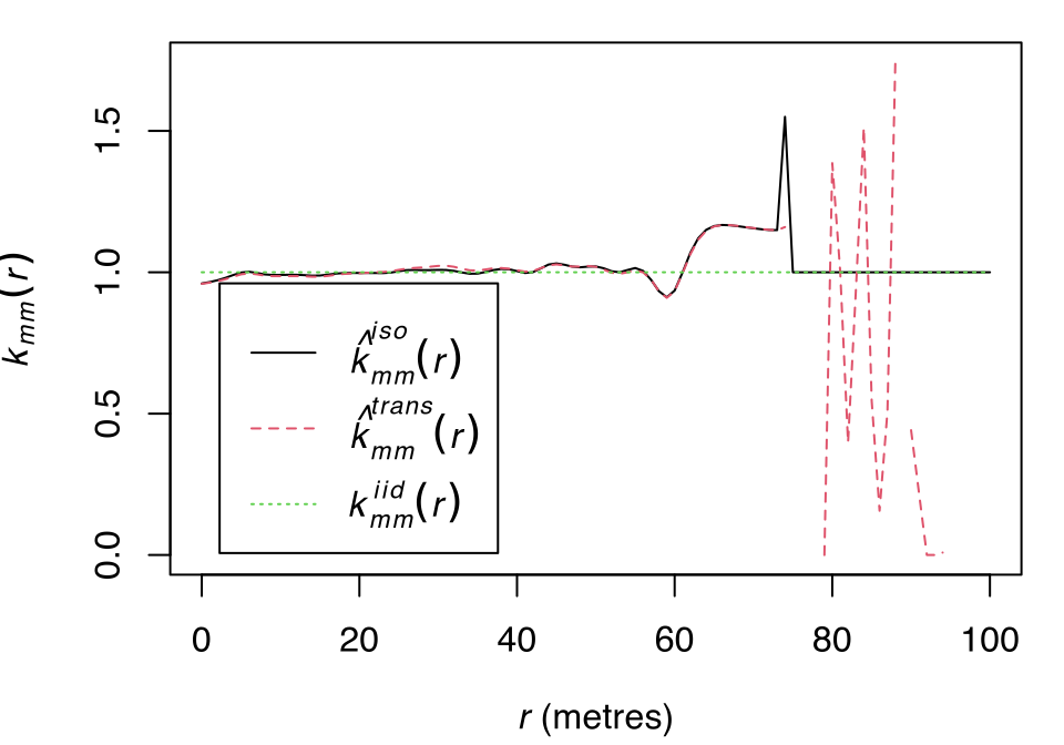
The S3 method .illegal2theo.fv() (Listing 19.21) replaces the recommended function values after the first illegal \(r\) (Section 19.5) of the malformed function-value-table fv_mal (Listing 19.17) with its theoretical values (Figure 19.4).
Listing 19.21: Advanced: function .illegal2theo.fv() (Listing 19.17)
par(mar =c(4, 4, 1, 1))fv_mal |>.illegal2theo() |> spatstat.explore::plot.fv(xlim =c(0, 100), main =NULL)# r≥75.0 replaced with theo
Figure 19.4: Replaces with theoretical values after the first illegal \(r\) (Listing 19.17)
Listing 19.23 creates the toy examples of a coarse and a fine function-value-table at a coarse and a fine\(r\)-vector for the mark correlation of the point-pattern spruces (Section 9.21).
Listing 19.23: Data: coarse versus fine function-value-table
r =list(coarse =0:9,fine =seq.int(from =0, to =9, by = .01))sprucesK = r |>lapply(FUN = \(r) { spatstat.data::spruces |> spatstat.explore::markcorr(r = r) })
Listing 19.24: Figure: coarse versus fine function-value-table, trapezoidal integration (Listing 19.23)
Figure 19.6: coarse versus fine function-value-table, trapezoidal integration (Listing 19.23)
19.6.1 Interpolation
19.6.1.1 Linear Interpolation
Function approxfun.fv() creates a linear interpolation from a function-value-table and returns an R object of S3 class 'function'. This is a “pseudo” S3 method, as the workhorse function stats::approxfun() is not an S3 generic function.
Function splinefun.fv() creates a spline interpolation from a function-value-table and returns an R object of S3 class 'function'. This is a “pseudo” S3 method, as the workhorse function stats::splinefun() is not an S3 generic function.
Function interpSpline_.fv() creates a B-spline or a piecewise polynomial spline interpolation from a function-value-table and returns an R object of S3 class 'spline'. This is a “pseudo” S3 method, as the parameterization of the workhorse S3 generic function splines::interpSpline() is not ideal for this purpose.
Function loess.fv() creates a local polynomial regression fit from a function-value-table and returns an R object of S3 class 'loess'. This is a “pseudo” S3 method, as the workhorse function stats::loess() is not an S3 generic function.
Function ksmooth.fv() creates a kernel regression smoother from a function-value-table and returns an R object of S3 class 'ksmooth'. This is a “pseudo” S3 method, as the workhorse function stats::ksmooth() is not an S3 generic function.
Function smooth.spline.fv() creates a smoothing spline from a function-value-table and returns an R object of S3 class 'smooth.spline'. This is a “pseudo” S3 method, as the workhorse function stats::smooth.spline() is not an S3 generic function.
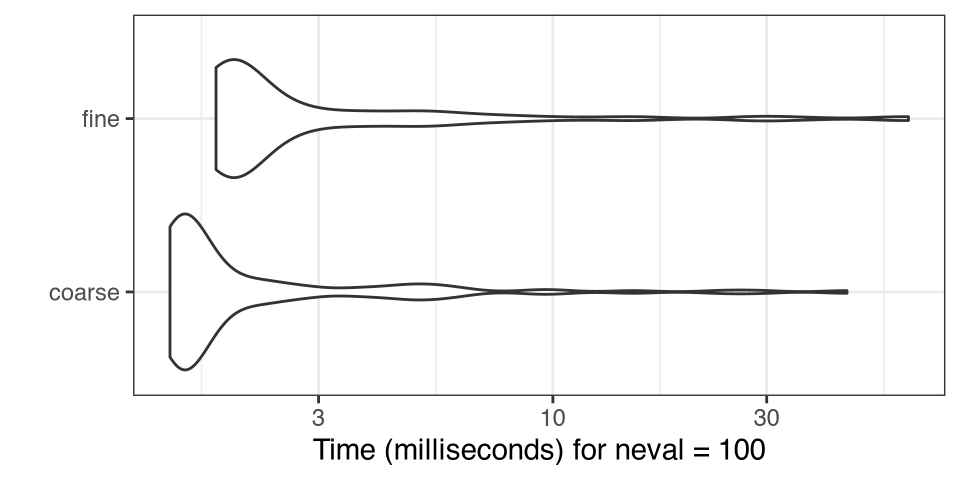
An experienced reader may wonder: is it truly advantageous to compute a coarse function-value-table sprucesK$coarse and then perform interpolation (Section 19.6.1) and/or smoothing (Section 19.6.2), rather than computing a fine function-value-table sprucesK$fine to start with? This is an excellent question! As of package spatstat.explore (v3.7.0.4), we observe only minor increase in the computation time of the creation of a function-value-table, even when the grid of the \(r\)-vector is 100 times finer (Listing 19.35, Figure 19.14) via package microbenchmark(Mersmann 2024, v1.5.0). This observation justifies the use of the plain-and-naïve trapezoidal integration (Chapter 10, Section 10.2) on a fine function-value-table (Figure 19.6, Right), rather than employing more sophisticated numerical integration methods, e.g., the Simpson’s rulepracma::simpson(), the adaptive Simpson quadraturepracma::quad(), etc. on an interpolation and/or smoothing of a coarse function-value-table.
Listing 19.35: Benchmark: coarse versus fine function-value-table (Listing 19.23)
suppressPackageStartupMessages(library(spatstat))microbenchmark::microbenchmark(coarse =markcorr(spruces, r = r$coarse),fine =markcorr(spruces, r = r$fine)) |> microbenchmark:::autoplot.microbenchmark() + ggplot2::labs(title =NULL) + ggplot2::theme_bw()
Figure 19.14: Benchmarks (Mersmann 2024): coarse versus fine function-value-table